Initial Value Problem#
강좌: 수치해석
Initial Value Problem#
초기 조건이 주어진 상미분 방정식은 다음과 같이 표현할 수 있다.
시간 \(t\) 에서 해를 구하기 위해서는 미분방정식을 적분해서 구할 수 있다.
Explicit Euler Method#
Taylor Series를 이용하면 다음과 같이 근사할 수 있다.
시간 \(t_n\) 일 때 \(y\)를 \(y_n\) 이고 시간 간격 \(h=\Delta t\) 로 하면 다음과 같이 근사할 수 있다.
정확도#
수치해석시 오차는 다음과 같다.
Trunaction Error
Round-off Error
Local truncation error (LTE)
Euler 기법의 경우 매 시간마다 오차가 발생한다.
LTE가 누적되어 Global truncation error가 된다.
Taylor Expansion 적용하면
\[ y_{n+1} = y_n + h \frac{dy}{dt} + \frac{h^2}{2!} \frac{d^2y}{dt^2} + O(h^3) \]즉 오차는 다음과 같다.
\[ E_t = \frac{h^2}{2!} \frac{d^2y}{dt^2} + O(h^3) = O(h^2). \]전 시간 영역에 대해서 오차가 누적되므로 1차 정확도 (\(O(h)\))가 된다.
Revisit 수치해석 101#
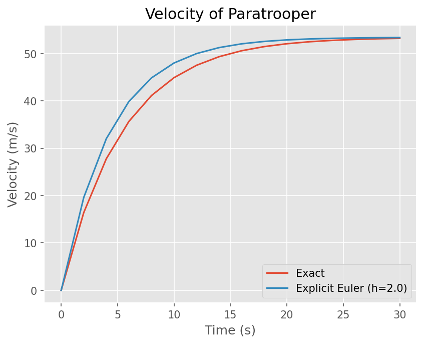
낙하산병 문제 는 다음과 같다.
여기서 낙하산병 몸무게 \(m=68.1 kg\), 항력계수 \(c=12.5kg/s\) 그리고 중력가속도 \(g=9.81 kg/s\) 이다.
%matplotlib inline
from matplotlib import pyplot as plt

import numpy as np

plt.style.use('ggplot')
plt.rcParams['figure.dpi'] = 150
# 주요 상수
m, c, g = 68.1, 12.5, 9.81

# 우변 함수 작성
def f(t, v):
    return g - c/m*v
# 엄밀해 계산 함수
def exact(t):
    return g*m/c*(1-np.exp(-(c/m)*t))
# 시간간격
h = 2.0

# 최종 시간
te = 30

# 초기조건
v0 = 0

# 계신 시간 간격
t = np.arange(0, te, h)

# Add Last points
t = np.insert(t, len(t), te)

# Array for solution
y = np.empty_like(t)
y[0] = v0

for i, ti in enumerate(t):
    if i < len(y) - 1:
        y[i+1] = y[i] + h*f(ti, y[i])
# Plot Exact solution and Numerical solution
plt.plot(t, exact(t))
plt.plot(t, y)

# 그래프 선 이름
plt.legend(['Exact', 'Explicit Euler (h={})'.format(h)])

# x,y 축 이름
plt.xlabel('Time (s)')
plt.ylabel('Velocity (m/s)')

# 그래프 이름
plt.title('Velocity of Paratrooper')
Text(0.5, 1.0, 'Velocity of Paratrooper')
DIY #1#
Euler 기법을 계산하는 함수를 구현하시오. \(h\) 값을 0.2, 0.5, 1.0, 2.0, 5.0, 10.0 으로 바꿔보면서 결과를 확인하시오.
# Your Answer
def explicit_euler(f, tspan, y0, dt):
    """
    Explicit Euler Method

    Parameter
    ---------
    f : function
        Derivative
    tspan : tuple
        Initial and final time ex) (ti, te)
    y0 : float
        Initial solution
    dt: float
        Time step size

    Return
    ------
    t : array
        Time series
    y : array
        solutions
    """
    # Write your Code (Delete below pass)
    return t, y
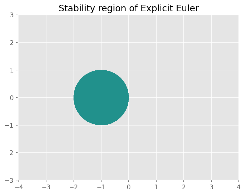
안정성#
시간 간격에 따라 정확도 뿐 아니라 알고리즘이 발산할 수 있다. 이는 수치 안정성과 관계된다.
안정성을 분석하기 위해 Model problem을 생각한다.
\(\lambda_R < 0\) 인 경우 이 미분방정식은 해가 제한되어 (bounded) 있다.
Explicit Euler에 적용하면 다음과 같다.
즉
여기서 \(|\sigma| < 1\) 일 때 수치 기법의 해가 발산하지 않는다.
# Make grid
x = np.linspace(-3, 3, 201)
y = np.linspace(-3, 3, 201)
X, Y = np.meshgrid(x, y)
z = X + Y*1j

# Amplication factor of Explicit Euler (z=lambda h)
sig = 1 + z

# Same scale of x and y
plt.axis('equal')

# Stability region
plt.contourf(X,Y,abs(sig), levels=[0, 1])

# Title
plt.title('Stability region of Explicit Euler')
Text(0.5, 1.0, 'Stability region of Explicit Euler')
낙하산 병 문제#
\(\lambda = c/m \approx 0.1836 \) 이므로
즉 \(h < m/c= 10.89\) 범위에서만 안정하다.
Explicit Euler 개선#
Heun’s Method#
미분 기울기를 \(t_n\) 일 때 값과 \(t_{n+1}\) 일 때 예측값으로 보정한다.
Predictor step
\[ \tilde{y}_{n+1} = y_n + h f(t_n, y_n) \]Corrector step
\[ y_{n+1} = y_n + h \frac{f(t_n, y_n) + f(t_n, \tilde{y}_{n+1})}{2} \]

Fig. 21 Heun’s Method (from Wikipedia)#
# 시간간격
h = 2.0

# 최종 시간
te = 30

# 초기조건
v0 = 0

# 계신 시간 간격
t = np.arange(0, te, h)

# Add Last points
t = np.insert(t, len(t), te)

# Array for solution
y = np.empty_like(t)
y[0] = v0

for i, ti in enumerate(t):
    if i < len(y) - 1:
        yt = y[i] + h*f(ti, y[i])
        y[i+1] = y[i] + 0.5*h*(f(ti, y[i]) + f(ti, yt))
# Plot Exact solution and Numerical solution
plt.plot(t, exact(t))
plt.plot(t, y)

# 그래프 선 이름
plt.legend(['Exact', 'Heun (h={})'.format(h)])

# x,y 축 이름
plt.xlabel('Time (s)')
plt.ylabel('Velocity (m/s)')

# 그래프 이름
plt.title('Velocity of Paratrooper')
Text(0.5, 1.0, 'Velocity of Paratrooper')

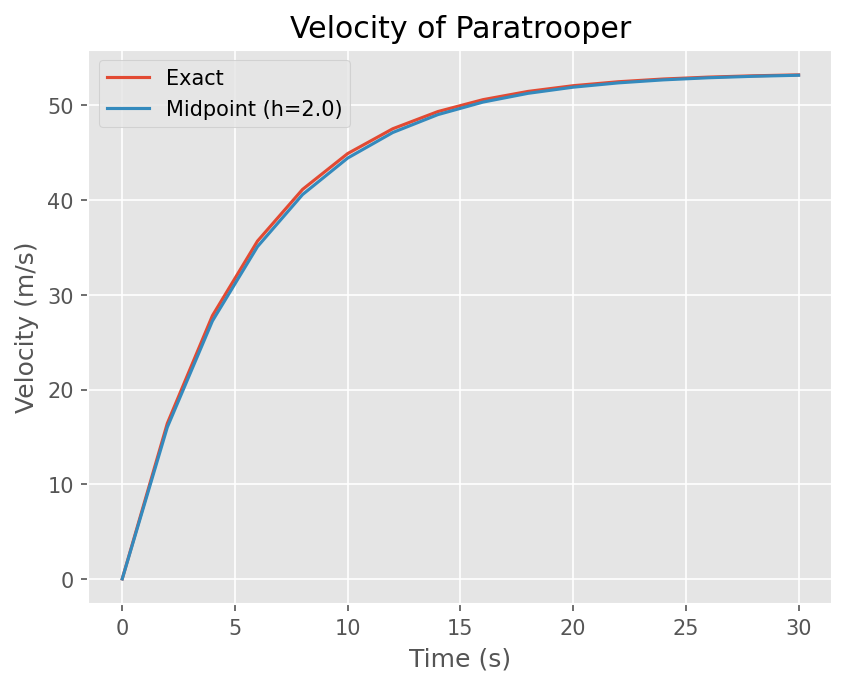
Midpoint Method#
중앙점 \(y_{n+1/2}\) 에서 기울기를 이용하는 방법이다. 중앙점에서 값은 Euler Method로 예측한다.

Fig. 22 Midpoint Method (from Wikipedia)#
# 시간간격
h = 2.0

# 최종 시간
te = 30

# 초기조건
v0 = 0

# 계신 시간 간격
t = np.arange(0, te, h)

# Add Last points
t = np.insert(t, len(t), te)

# Array for solution
y = np.empty_like(t)
y[0] = v0

for i, ti in enumerate(t):
    if i < len(y) - 1:
        yh = y[i] + 0.5*h*f(ti, y[i])
        y[i+1] = y[i] + h*f(ti+0.5*h, yh)
# Plot Exact solution and Numerical solution
plt.plot(t, exact(t))
plt.plot(t, y)

# 그래프 선 이름
plt.legend(['Exact', 'Midpoint (h={})'.format(h)])

# x,y 축 이름
plt.xlabel('Time (s)')
plt.ylabel('Velocity (m/s)')

# 그래프 이름
plt.title('Velocity of Paratrooper')
Text(0.5, 1.0, 'Velocity of Paratrooper')
DIY #2#
Heun’s method, Midpoint method 로 ODE를 해석하는 함수를 구현하시오. \(h\) 값을 0.2, 0.5, 1.0, 2.0, 5.0, 10.0 으로 바꿔보면서 결과를 확인하시오.
함수의 입출력은 위의 Explicit Euler와 같다
더 정확한 Explicit Method#
정확도를 높이기 위해서 2가지 방법이 고려된다.
Multi-stage method
한 시간 간격 (step) 을 전진하기 위해 여러 Stage를 계산함
Multi-step method
한 시간 간격을 전진하기 위해 이전 여러 step의 결과를 활용함
이들은 모두 Taylor expansion에서 고차항을 근사한다.
Runge-Kutta Method#
Multi-stage 기법에 대표적인 방법으로 다음과 같은 과정으로 계산한다.
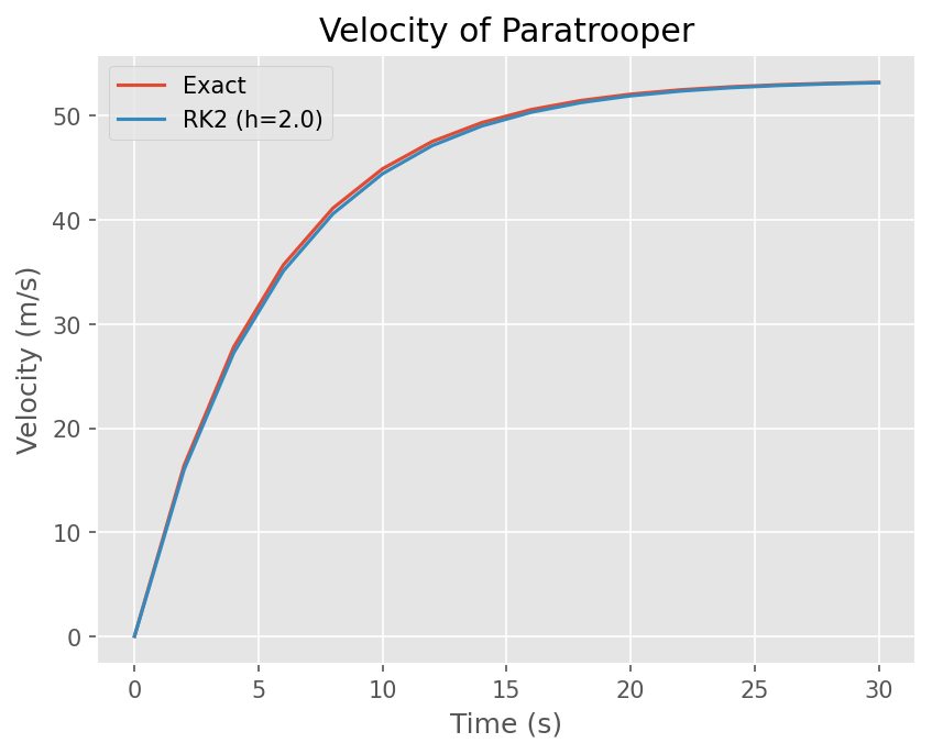
2차 Runge-Kutta Method#
2차 Runge Kutta 기법은 다음과 같다.
계수 관계식 유도#
\(y\) 에 대한 Taylor 전개는 다음과 같다.
여기서 \(f'(t_n, y_n)\) 은 다음과 같이 Chain rule을 적용해서 계산할 수 있다.
이를 적용하면 다음과 같다.
2차 Runge Kutta 식을 정리하면 다음과 같다.
위 두 식을 비교하면 다음 관계를 얻는다.
이를 만족하는 계수는 무수히 많다. 즉 무수히 많은 2차 Runge Kutta 법이 있다.
Butcher tableau#
Runge Kutta 기법의 계수는 다음 Butcher tableau로 표기한다.
2차 Runge Kutta 기법의 계수는 다음과 같이 표현할 수 있다.
이전에 배운 Heun’s method, Midpoint 기법 모두 2차 Runge Kutta의 종류이며 다음과 같이 표현할 수 있다.
Huen’s method
\[\begin{split} \begin{array}{c|cc} 0 & 0 & \\ 1 & 1 & 0 \\ \hline & 1/2 & 1/2 \end{array} \end{split}\]Midpoint method
\[\begin{split} \begin{array}{c|cc} 0 & 0 & \\ 1/2 & 1/2 & 0 \\ \hline & 0 & 1 \end{array} \end{split}\]
Richardson 법은 절단오차를 최소화 하기 위해 \(b_2=2/3\) 로 한 기법이다.
Richardson method
\[\begin{split} \begin{array}{c|cc} 0 & 0 & \\ 3/4 & 3/4 & 0 \\ \hline & 1/3 & 2/3 \end{array} \end{split}\]
# 시간간격
h = 2.0

# 최종 시간
te = 30

# 초기조건
v0 = 0

# 계신 시간 간격
t = np.arange(0, te, h)

# Add Last points
t = np.insert(t, len(t), te)

# Array for solution
y = np.empty_like(t)
y[0] = v0

for i, ti in enumerate(t):
    if i < len(y) - 1:
        k1 = f(ti, y[i])
        k2 = f(ti + 3/4*h, y[i] + 3/4*k1*h)
        y[i+1] = y[i] + h*(k1 + 2*k2)/3
# Plot Exact solution and Numerical solution
plt.plot(t, exact(t))
plt.plot(t, y)

# 그래프 선 이름
plt.legend(['Exact', 'RK2 (h={})'.format(h)])

# x,y 축 이름
plt.xlabel('Time (s)')
plt.ylabel('Velocity (m/s)')

# 그래프 이름
plt.title('Velocity of Paratrooper')
Text(0.5, 1.0, 'Velocity of Paratrooper')
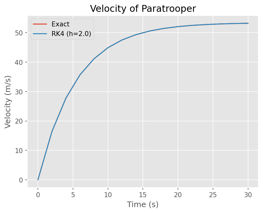
4차 Runge-Kutta Method#
가장 많이 쓰이는 4차 Runge Kutta 기법은 다음과 같다.
# 시간간격
h = 2.0

# 최종 시간
te = 30

# 초기조건
v0 = 0

# 계신 시간 간격
t = np.arange(0, te, h)

# Add Last points
t = np.insert(t, len(t), te)

# Array for solution
y = np.empty_like(t)
y[0] = v0

for i, ti in enumerate(t):
    if i < len(y) - 1:
        k1 = f(ti, y[i])
        k2 = f(ti + 1/2*h, y[i] + 1/2*k1*h)
        k3 = f(ti + 1/2*h, y[i] + 1/2*k2*h)
        k4 = f(ti + h, y[i] + k3*h)
        y[i+1] = y[i] + h*(k1 + 2*k2 + 2*k3 + k4)/6
# Plot Exact solution and Numerical solution
plt.plot(t, exact(t))
plt.plot(t, y)

# 그래프 선 이름
plt.legend(['Exact', 'RK4 (h={})'.format(h)])

# x,y 축 이름
plt.xlabel('Time (s)')
plt.ylabel('Velocity (m/s)')

# 그래프 이름
plt.title('Velocity of Paratrooper')
Text(0.5, 1.0, 'Velocity of Paratrooper')
DIY #3#
2차와 4차 Runge-Kutta 기법을 계산하는 함수를 만드시오.
함수의 입출력은 위의 Explicit Euler와 같다
다음 미분방정식을 구간 \([0, 4]\)에서 해석하시오. 초기값은 0이다. 시간간격은 \(h=0.1, 0.2, 0.5\) 에 대해 계산하시오.
Mutli-step Method#
Multi-stage 기법과 달리 이전 step (\(y_{n-1}, y_{n-2}...\)) 결과를 이용하여 정확도를 높히는 방법이다.
Not self-starting!!!
초기에 Explicit Euler 기법 등으로 이용하여 이전 Step 값을 구해야 함
Leapfrog method#
Central difference를 이용
\[ y_{n+1} - y_{n-1} = 2h f(t_n, y_n) + O(h^3) \]2차 정확도 기법
Stability
\(y_n = \sigma^n y_0\) 로 가정
\[ \sigma^{n+1} - \sigma_{n-1} = 2h\lambda \sigma^n \]2개의 해가 존재함
\[\begin{split} \begin{align} \sigma_1 &= \lambda h + \sqrt{\lambda^2 h^2 + 1} = 1 + \lambda h + \frac{1}{2} \lambda^2 h^2 + O(h^3) \\ \sigma_2 &= \lambda h - \sqrt{\lambda^2 h^2 + 1} =-1 + \lambda h - \frac{1}{2} \lambda^2 h^2 + O(h^3) \end{align} \end{split}\]첫번째 해는 2차 정확도를 만족함
두번째 해는 Spurious 해로, 불안정성 야기함
\(h\rightarrow 0\), \(\sigma_2 \ne 1\).
Pure imaginary \(\lambda = i \omega\)
\(\sigma_{1,2} = 1\), if \(|\omega h| \leq 1\).
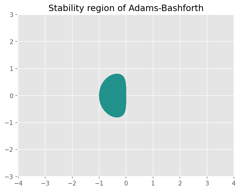
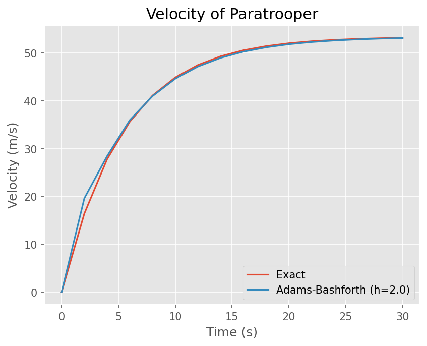
Adams-Bashforth method#
Taylor expansion 이용
\[ y_{n+1} = y_n + h \frac{dy}{dt} + \frac{h^2}{2!} \frac{d^2y}{dt^2} + \frac{h^3}{3!} \frac{d^3y}{dt^3} + O(h^4) \]\(y'_n=f(t_n, y_n)\) 이고, 후방차분 기법을 이용하면
\[ y''_n = \frac{f(t_n, y_n) - f(t_{n-1}, y_{n-1})}{h} + O(h) \]이 둘을 대입하면,
\[ y_{n+1} = y_n + \frac{3h}{2} f(t_n, y_n) - \frac{h}{2} f(t_{n-1}, y_{n-1}) + O(h^3) \]2차 정확도 기법
Stability 분석
\[\begin{split} \begin{align} \sigma_1 &= \frac{1}{2} \left ( 1 + \frac{3}{2} \lambda h + \sqrt{1 + \lambda h + \frac{9}{4} \lambda^2 h^2} \right ) = 1 + \lambda h + \frac{1}{2} \lambda ^2 h^2 + O(h^3) \\ \sigma_2 &= \frac{1}{2} \left ( 1 + \frac{3}{2} \lambda h - \sqrt{1 + \lambda h + \frac{9}{4} \lambda^2 h^2} \right ) = \frac{1}{2} \lambda h - \frac{1}{2} \lambda ^2 h^2 + O(h^3) \end{align} \end{split}\]Spurious 해가 존재하나 덜 위험함.
\(h\rightarrow 0\), \(\sigma_2 = 0\).
# Make grid
x = np.linspace(-3, 3, 201)
y = np.linspace(-3, 3, 201)
X, Y = np.meshgrid(x, y)
z = X + Y*1j

# Amplication factor of Explicit Euler (z=lambda h)
sig1 = 0.5*(1 + 3/2*z + np.sqrt(1 + z + 9/4*z**2))
sig2 = 0.5*(1 + 3/2*z - np.sqrt(1 + z + 9/4*z**2))

# Same scale of x and y
plt.axis('equal')

# Stability region
plt.contourf(X,Y, np.maximum(abs(sig1), abs(sig2)), levels=[0, 1])

# Title
plt.title('Stability region of Adams-Bashforth')
Text(0.5, 1.0, 'Stability region of Adams-Bashforth')
# 시간간격
h = 2.0

# 최종 시간
te = 30

# 초기조건
v0 = 0

# 계신 시간 간격
t = np.arange(0, te, h)

# Add Last points
t = np.insert(t, len(t), te)

# Array for solution
y = np.empty_like(t)
y[0] = v0

for i, ti in enumerate(t):
    # Compute f(t_{i}, y_{i})
    fn = f(ti, y[i])

    if i == 0:
        # Starting by Explicit Euler
        y[i+1] = y[i] + h*fn

    elif i < len(y) - 1:

        y[i+1] = y[i] + 1.5*h*fn - 0.5*h*fm

    # Update fn as f(t_{i-1}, y_{i-1})
    fm = fn
# Plot Exact solution and Numerical solution
plt.plot(t, exact(t))
plt.plot(t, y)

# 그래프 선 이름
plt.legend(['Exact', 'Adams-Bashforth (h={})'.format(h)])

# x,y 축 이름
plt.xlabel('Time (s)')
plt.ylabel('Velocity (m/s)')

# 그래프 이름
plt.title('Velocity of Paratrooper')
Text(0.5, 1.0, 'Velocity of Paratrooper')
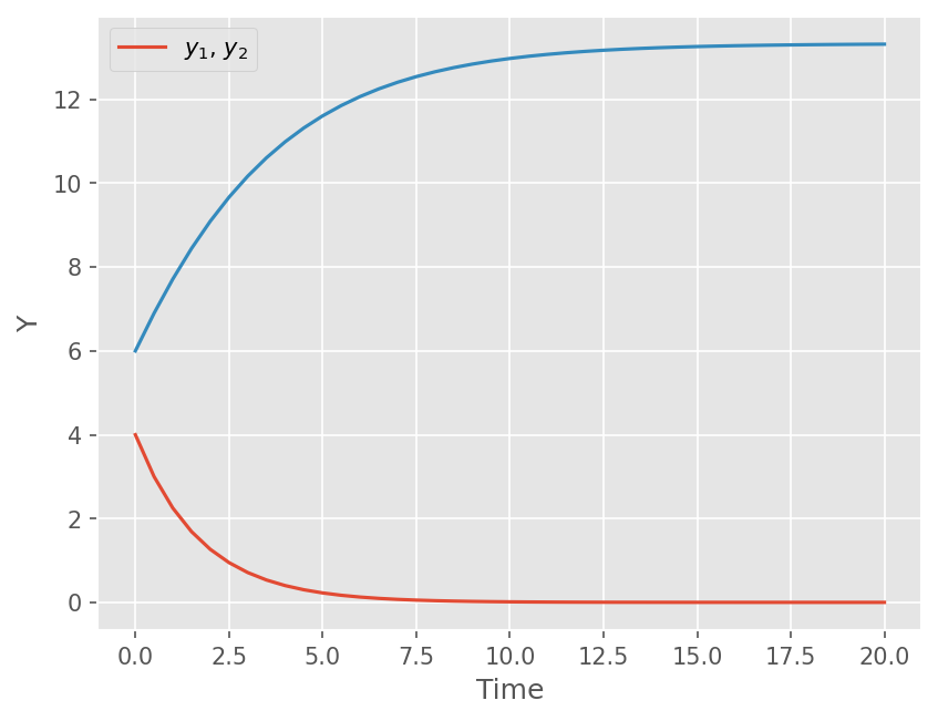
Systems of ODEs#
다음 문제를 생각해보자
초기조건은 \((y_1, y_2) = (4, 6)\) 이다.
이론적으로는 이 문제는 다음 행렬식으로 생각할 수 있다.
Explicit Euler method, Runge-Kutta method은 동일하게 적용할 수 있다. \(y\) 가 scalar 가 아닌 벡터로 생각한다.
# Derivative
def f(t, y):
    return np.array([-0.5*y[0], 4 - 0.3*y[1] - 0.1*y[0]])

# Initial condition
y0 = np.array([4, 6])
# 시간간격
h = 0.5

# 최종 시간
te = 20

# 초기조건
v0 = 0

# 계신 시간 간격
t = np.arange(0, te, h)

# Add Last points
t = np.insert(t, len(t), te)

# Array for solution
y = np.empty((len(y0), len(t)))
y[:, 0] = y0

for i, ti in enumerate(t):
    if i < len(t) - 1:
        y[:, i+1] = y[:, i] + h*f(ti, y[:, i])
# Plot y1, y2
plt.plot(t, y[0])
plt.plot(t, y[1])

plt.xlabel('Time')
plt.ylabel('Y')

plt.legend(['$y_1$, $y_2$'])
<matplotlib.legend.Legend at 0xf79ee674b750>
DIY 3#
앞서 만든 Explicit Euler, 2nd and 4th order Runge-Kutta 기법으로 ODE를 푸는 함수를 확장하시오.
시간 간격을 \(h=0.1, 0.25, 0.5, 1.0, 2.0, 4.0\) 으로 바꿔보면서 계산하시오.
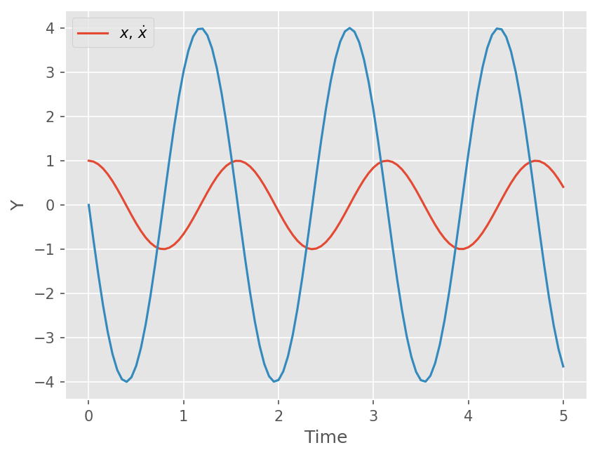
High-order ODE#
다음 Spring-Mass 문제를 생각하자.
즉
이러한 고차 ODE를 해석하기 위해서는 다음과 같이 연립 1계 미분방정식으로 만든다.
예제#
\(m=1, k=16\) 이고 \(x_0 = 1\), \(\dot{x}_0=0\) 일 때 수치적으로 해석하시오.
m, k = 1, 16

# Derivative
def f(t, y):
    return np.array([y[1], -k/m*y[0]])

# Initial condition
y0 = np.array([1, 0])
# 시간간격
h = 0.05

# 최종 시간
te = 5.0

# 계신 시간 간격
t = np.arange(0, te, h)

# Add Last points
t = np.insert(t, len(t), te)

# Array for solution
y = np.empty((len(y0), len(t)))
y[:, 0] = y0

for i, ti in enumerate(t):
    if i < len(t) - 1:
        k1 = f(ti, y[:, i])
        k2 = f(ti + 1/2*h, y[:, i] + 1/2*k1*h)
        k3 = f(ti + 1/2*h, y[:, i] + 1/2*k2*h)
        k4 = f(ti + h, y[:, i] + k3*h)
        y[:, i+1] = y[:, i] + h*(k1 + 2*k2 + 2*k3 + k4)/6
# Plot y1, y2
plt.plot(t, y[0])
plt.plot(t, y[1])

plt.xlabel('Time')
plt.ylabel('Y')

plt.legend([r'$x$, $\dot{x}$'])
<matplotlib.legend.Legend at 0xf79ee64cbc50>
DIY 4#
연립 ODE를 해석하는 Explicit Euler, 2nd and 4th order Runge-Kutta 기법 함수를 이용하여 이 문제를 풀어보시오.
시간 간격을 \(h=0.01, 0.05, 0.1\) 로 바꿔가며 풀어보시오.
DIY 5#
앞서 해석한 낙하산병 문제에서 낙하 거리도 같이 계산하시오. 자유낙하일때와 비교하시오.
Scipy 활용#
scipy.integrate 모듈은 수치 적분과 관련된 다양한 알고리듬을 제공한다.
참고
Initial value problem#
solve_ivp 함수는 다양한 고성능 Multi-stage 및 Multi-step method를 제공한다. 특히 Adaptive time step을 지원하므로 시간 간격을 알아서 조정한다.